For Shits and Giggles: Optimized Sequential Sampling from Multiple Sensors (Arduino)
- By Peter Crona
- February 27, 2021
- technology
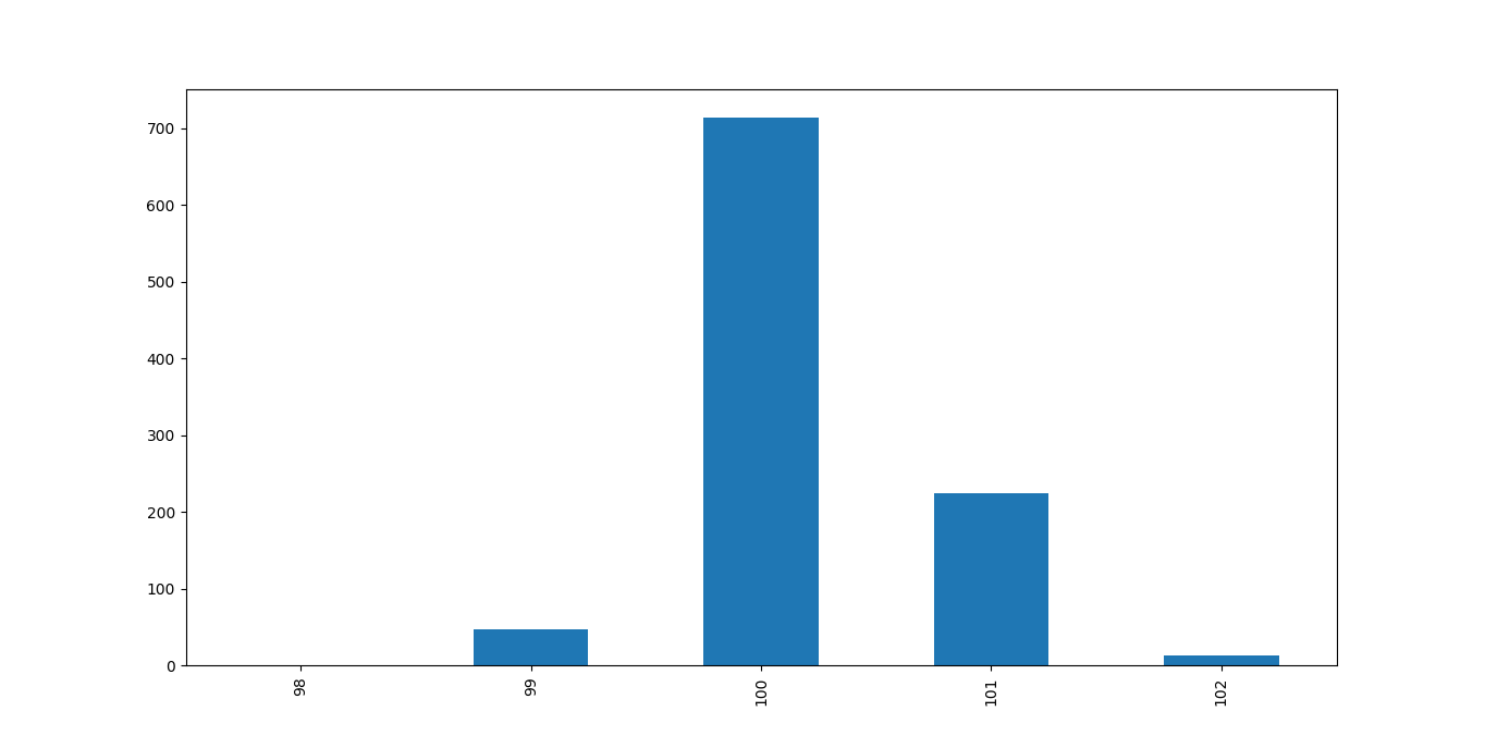
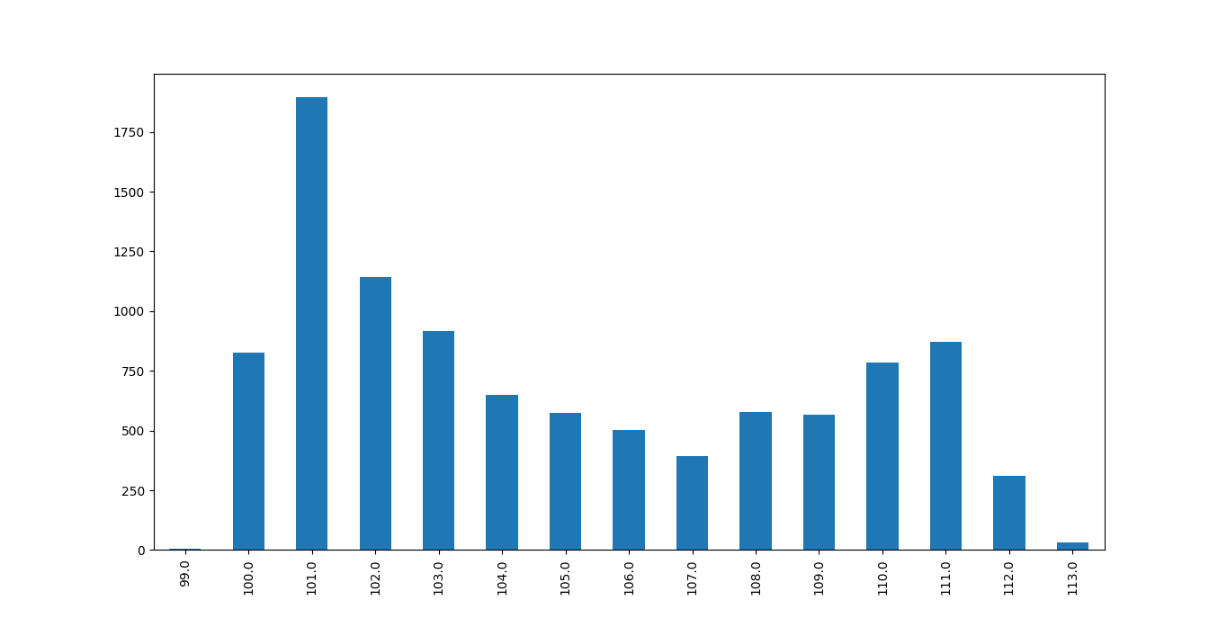
I woke up with a nice idea of how I’d use statistics and optimization to improve the precision when measuring pollutants by taking just the right number of samples. Turns out that sensors, at least those I have, give a fairly stable voltage, making it enough to spend a few milliseconds to take 30 samples per sensor or so to get a very stable value, and you’d get pretty good results with just one sample as well. An example of the distribution when sampling from a sensor (for around a second) can be seen in figure 1.
Not into natural language? Jump straight to the code!
Nevertheless, I still continued with the idea, as it is still a nice little project for practicing some C++ (currently reading A Tour of C++) as well as brushing up some statistics and optimization skills. I’m still hopeful that this can come in handy later for future projects, as so many problems we solve are just other problems in disguise anyway.
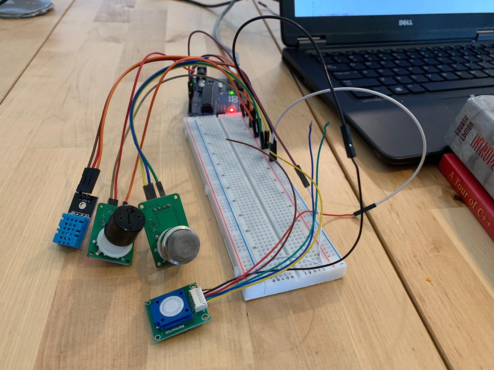
The problem at hand is that I want to measure the analog output from sensors. My fear was that it would be unstable, because I’ve seen it happen a few times. However, it appears to not be a big problem, as I generally get a standard deviation of around 0.5. My sensor setup can be seen in figure 2, it consists of sensors for measuring ozone, humidity and temperature.
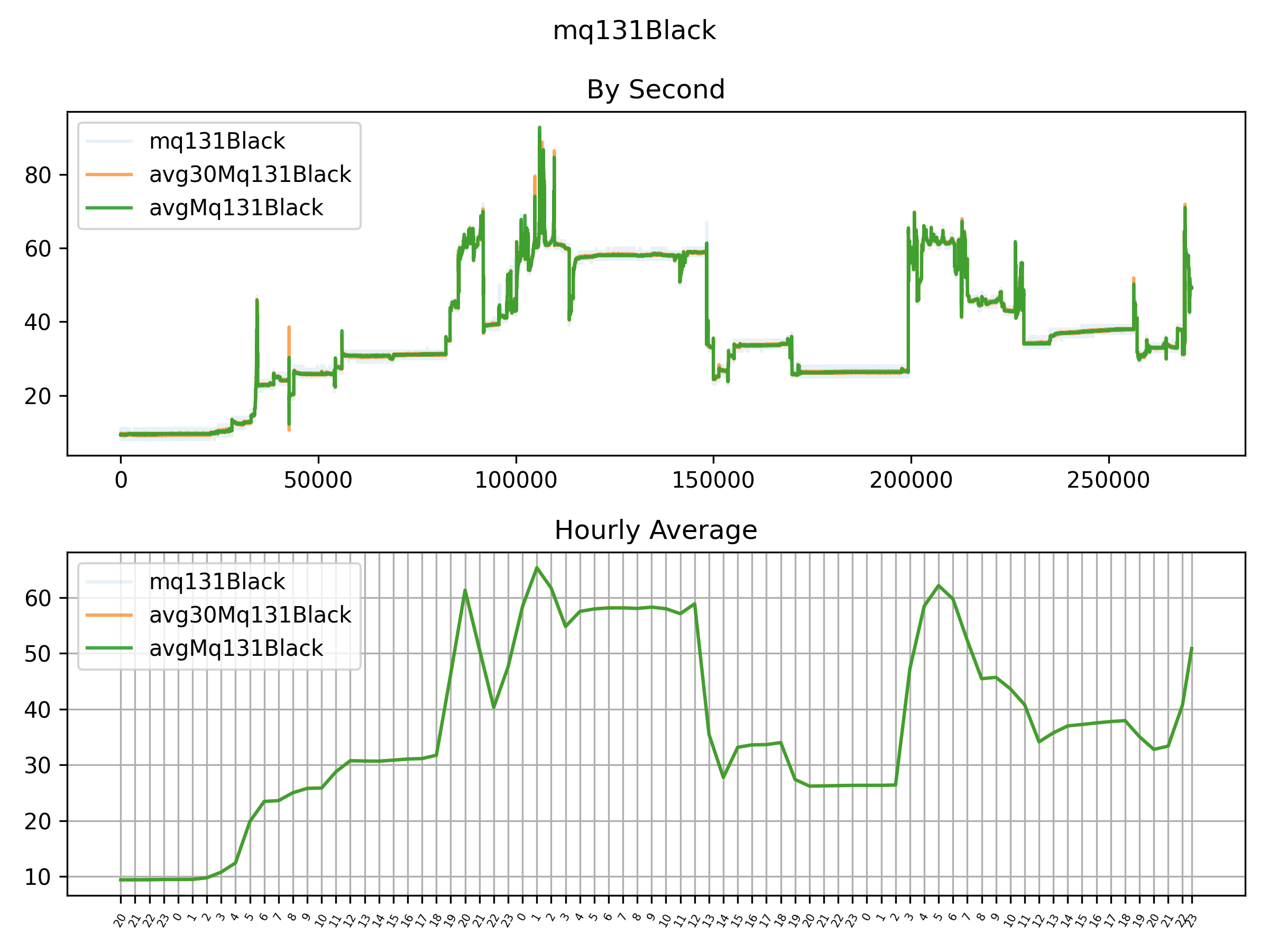
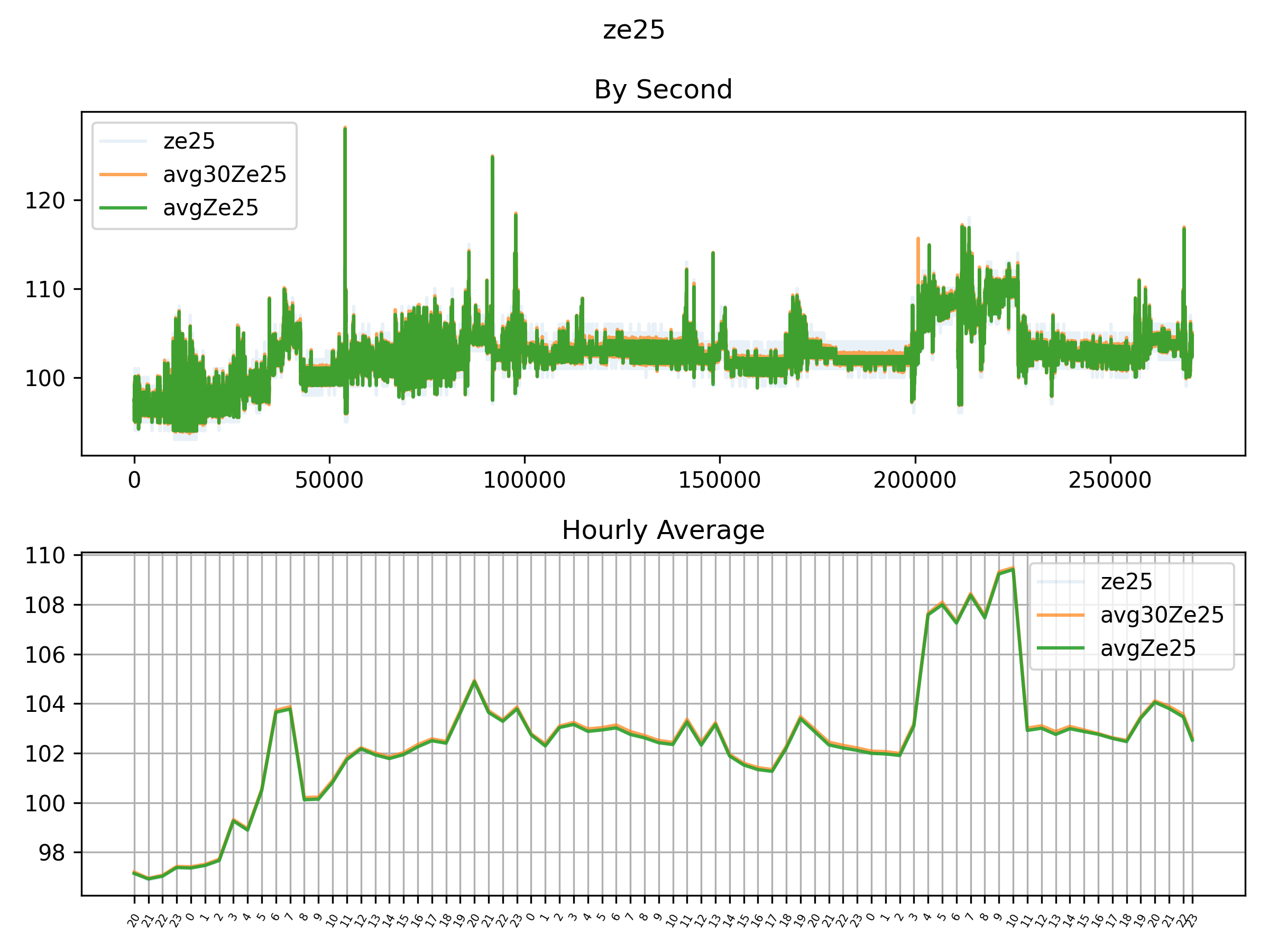
I wanted to present you with a messy graph of the black MQ131’s analog output. Now when I think about it, perhaps I did see messy data because it was not “burned in” - it is often specified in sensors’ data sheets that the sensor needs to be turned on for a few days if it has been unused for long or never used. Nevertheless, by using an appropriate scale for the Y-axis, we can still make it look messy as in figure 3.
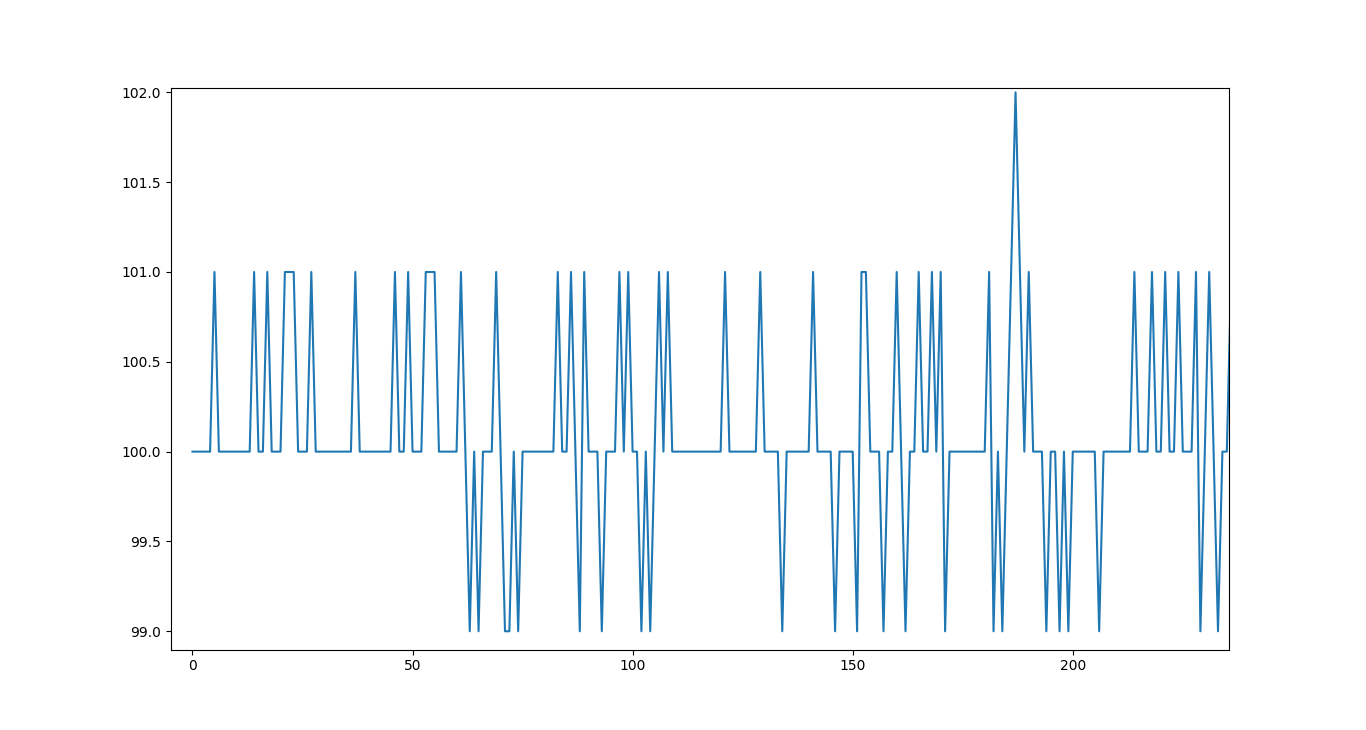
Rather than the jumpy voltage values in fig. 3, which is likely “noise” rather than true variations in O3 measurement, we’d prefer something as shown in fig. 4.
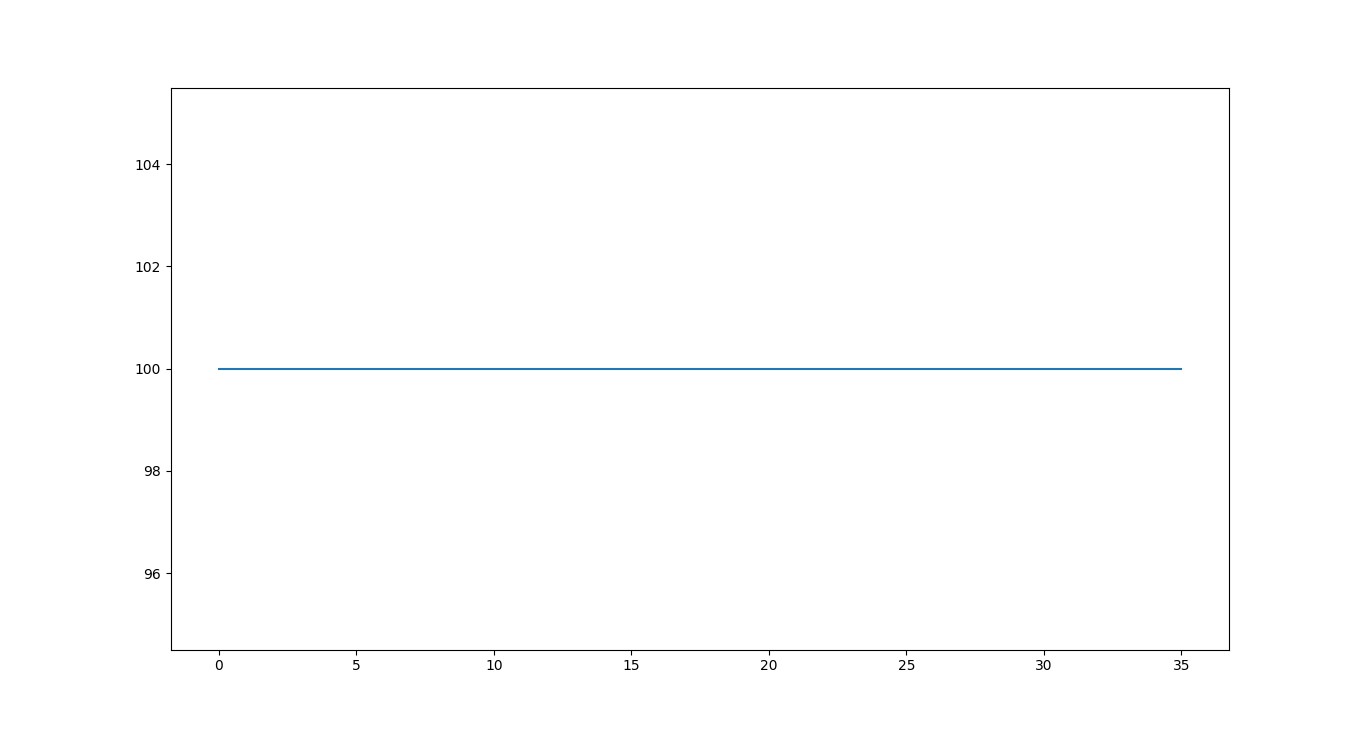
In figure 4 we get a completely flat line by simply taking the average of groups of 30 samples and rounding. The idea is that we can get rid of noise in this way by assuming that the ozone concentration is constant (well, that any changes are below our sensor’s resolution) in the time interval we’re working with (eg. 1s).
On one hand, we could just take 30 samples and be fine with that, but on the other hand, it’s more fun and more of a learning experience to try something different. After a bit of thinking, I formulated my problem as:
I want to sample for a fairly short time and get a decent estimate of the real concentration of the gas under investigation. Under the assumption that the sensor does do its job, but is just suffering from some noise in the measurements.
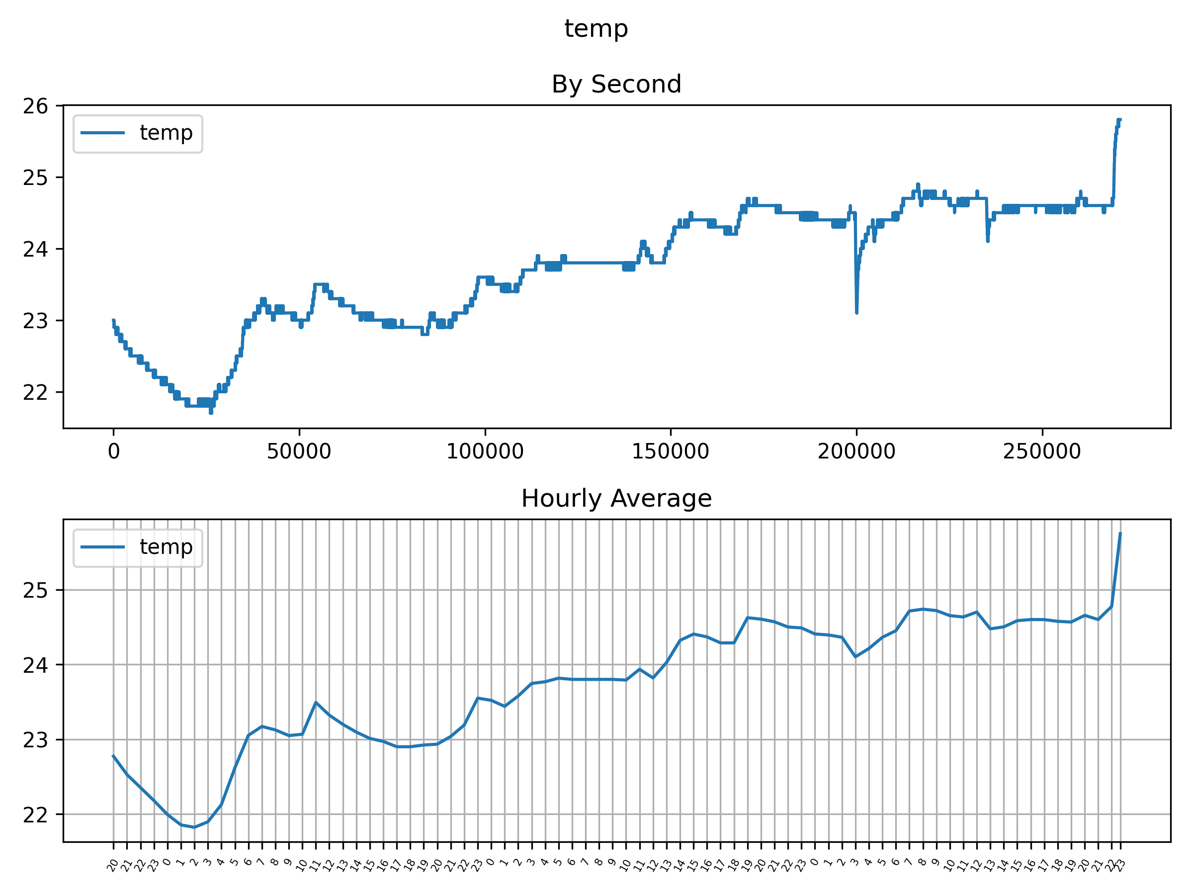
The “a fairly short time” comes from that I want to capture changes ASAP, because the concentration might change (truth to be told, I’m also impatient when measuring), an example of this is shown in figure 5, where we no longer have one “top”. Not sampling for too long is particularly important for me because I want to measure many things. For a starter, humidity, temperature and ozone, but hopefully will add nitrogen dioxide, particles, VOC and formaldehyde to that. All of this I would do simultaneously in an ideal world, as I want to explore the relation between different pollutants later. Furthermore, I want the ability to compare multiple sensors that measure the same thing.
To make things easier, I started to see the problem as a statistical problem:
There’s a true mean for the concentration in a specific time interval (eg. second). How can we model the quality of our estimate?
Brushing up on some stats skills [1] [2] quickly led me to confidence intervals and in particular margin of error. Assuming that all sensors are equally important, we can minimize the sum of the margin of error for all sensors, subject to a time budget (eg. 1 second) with a fixed desired confidence level (eg. 95%).
With all those ideas we can now break down our problem:
- Get a good estimate of the standard deviation for each sensor in a second.
- Calculate time to sample, so we can see how many samples we afford with a fixed maximum sampling time.
- Formulate optimization problem so some solver can solve it (future challenge might be to solve it ourselves in C++ - might be handy to recalculate from time).
The optimization problems will look something like:
$$
\begin{alignat}{2}
&\!\min_{n_x,\ x \in \text{sensors}} &\,& \sum_{x \in \text{sensors}} \frac {s_{x}} {\sqrt{n_{x}}} \\
\\
&\text{subject to} & & \sum_{x\in\text{sensors}} n_x <= \text{timeBudget} \\
\\
&\rlap{s_x\text{: estimated standard deviation of sensor x}} \\
&\rlap{n_x\text{: nr of samples from sensor x}} \\
\end{alignat}
$$
Basically, we want to minimize the sum of the margin of error of all sensors. The margin of error is actually given by:
$$t * \frac s {\sqrt{n}}\\$$
where the t is a constant given the chosen confidence level (eg. 95%) and degrees of freedom defined by the sample size (you just look it up in a table). As it won’t affect our optimization problem, we can simply drop it.
Solving such an optimization problem is a piece of cake for something like WolframAlpha, so after a bit of coding we get:
min (0.52 / sqrt(a) + 0.28 / sqrt(b) + 0.51 / sqrt(c)) s.t. a + b + c <= 8606
To which WolframAlpha responds:
(a, b, c)≈(3252.96, 2141.52, 3211.44)
As expected, we’re asked to sample less from the sensor with the lowest standard deviation. Keep in mind that we get one or more local minima from WolframAlpha. To perhaps make it easier to grasp, consider if we have a lot fewer samples and greater difference in standard deviations. We want to ask three questions to random people out on the street and we happen to know (lucky us!) that they have standard deviations 100, 500 and 2000. We are only allowed to ask 100 questions in total. That would give:
min (100 / sqrt(a) + 500 / sqrt(b) + 2000 / sqrt(c)) s.t. a + b + c <= 100
WolframAlpha kindly finds a local minima at:
(8.85576, 25.8944, 65.2498)
So, when walking around on the streets in your beautiful city, you’d ask question one 9 times, question two 26 times and question three 65 times. You’d end up with a summed “margin of error” of roughly 379, as opposed to roughly 452 if you’d split how many times you ask each question evenly. For question one, you’d notice that people tend to answer roughly the same, whereas for question three, you see very different answers. So you feel confident that you know roughly what to expect for question one pretty early, but for question three not so much.
As already pointed out, it turned out that we didn’t need to consider the confidence level. However, we could fix the margin of error and confidence level to something we want (eg. 0.5 with 95% confidence), and calculate the number of samples needed for that. This would in fact be easier, as we can simply use algebra to calculate the answer, as opposed to formulating and solving an optimization problem.
But let’s move on to actually using the results now, in its simplest form, we can just do something like this:
int samplesToTake[] {3253, 2142, 3211};
int nrSensors = sizeof(analogSensorReaderArray)
              / sizeof(analogSensorReaderArray[0]);
for (auto i = 0; i < nrSensors; i++) {
  StreamStats stats {};

  auto sensor = analogSensorReaderArray[i];
  for (auto j = 0; j < samplesToTake[i]; j++) {
    stats.reportNumber(sensor.read());
  }

  Serial.print(stats.average());
  Serial.print(",");
  Serial.print(sensor.read());
  Serial.print(",");
}

Serial.print(dht.readHumidity());
Serial.print(",");
Serial.print(dht.readTemperature());

Serial.println();
Where samplesToTake is just copy-pasted from WolframAlpha (and rounded).
As expected, given the low standard deviation, the difference is not massive. It is easiest to see for the MQ131 low concentration sensor (you might need to zoom in):
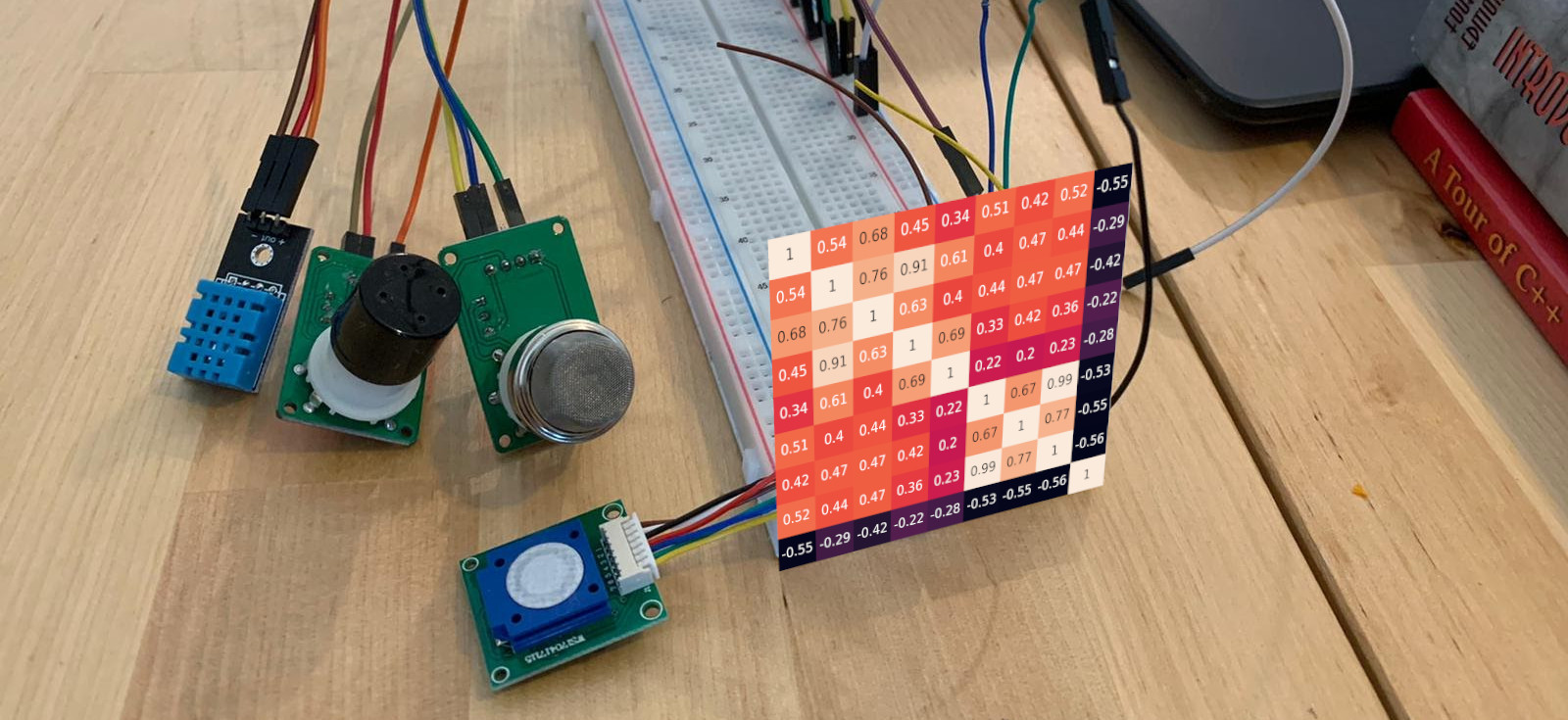
As we did sample from multiple sensors almost simultaneously, I can’t really resist looking at the correlation matrix:
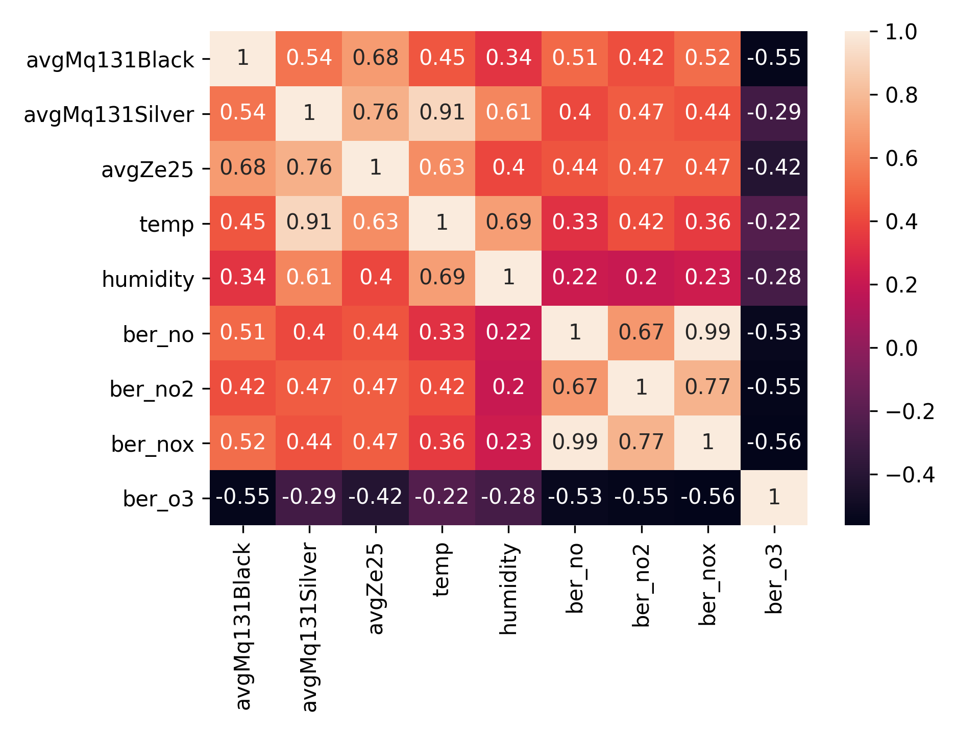
A pity is that we get a lower correlation between our Winsen ZE25-O3 sensor and Berlin’s NO2 measurements than in a previous experiment (0.60 VS 0.47). However, this might be explained by the correlation with temperature, as the temperature was pretty much rising throughout the whole measurement period. I also have some suspicions that Berlin’s air quality monitoring wasn’t working that well, for instance, it recently reported several hundreds μg/m3 of PM10 (which is quite a lot, even if sand that blew up from Sahara can explain elevated levels).
Interesting is to see that all sensors had negative correlation with outdoor ozone. I believe this can partly be explained by that ozone negatively correlates with NOx, and the sensors are sensitive to NOx which is simply dominating. So as O3 goes down and NOx goes up, we get a higher value. We can also see the high correlation with temperature. In fact, our MQ131 silver (high concentration ozone sensor) has a very strong correlation (0.91) with temperature. This perhaps is due to the fact that it isn’t made for measuring ambient ozone levels (so it basically figured the level was at zero), but still sensitive to temperature differences. Correlation matrices are awesome for forming a huge number of hypotheses (I’m a bit lazy here, of course, doesn’t hurt to look at the p-value to see how much you can trust the correlations too - for an example of that see my old post about Winsen ZE25-O3)!
Code
The code for the rest is available on Github. There’s not much going on beyond what was mentioned here. Perhaps slightly interesting is how the variance is calculated in StreamStats.cpp. The solution is inspired by a discussion at StackExchange which mentions a method from Donald Knuth’s book “The Art of Computer Programming”. I didn’t want memory to quickly become a limiting factor when setting the time budget (as we’re running this on an Arduino), and thus wanted to calculate the average and variance from a stream of values.
Conclusion
I showed how one can see sensor sampling as a statistical problem which in turn can be formulated as an optimization problem: we want to minimize the sum of all sensors’ margin of error subject to a time budget (maximum time we’re willing to sample). We then presented a solution where we estimate the standard deviation, calculate the number of samples we can take given our time budget and formulate an optimization problem in a format WolframAlpha understands, so that it can solve it for us. The solution shows how many samples each sensor should take.
Albeit this isn’t needed in exactly this shape - as just taking 30 samples per sensor seems to do the job - it was fun and I hope you, just as I, learnt something.
It is important to note that the methods used here were made up. If you are interested in a deeper dive, you might check out Statistical Sensor Calibration Algorithms, which I hope to find the time to read more carefully myself, to see whether I can apply any other ideas from there.
Future Work
I’m increasingly keen on looking at compensating for temperature and humidity. Basically see if I can increase the correlation with government sensors by assuming that humidity and temperature influence sensor voltage, and compensate for it. I’m a fan of machine learning and suspect it could help here.
Would also be interesting to look at solving the optimization problem in C++ (on the Arduino) so that it can perhaps recalibrate continuously (but also so that I can practice solving optimization problems). Based on the jumpy graph for the Winsen ZE25-O3 measurements, I suspect that perhaps the standard deviation did change a bit.
References
[1] L. Sullivan, Confidence Intervals. Boston University School of Public Health, [Online]. Available: https://sphweb.bumc.bu.edu/otlt/mph-modules/bs/bs704_confidence_intervals/bs704_confidence_intervals_print.html.
[2] J. S. Milton and J. C. Arnold, Introduction to probability and statistics: Principles and applications for engineering and the computing sciences. McGraw-Hill.